算法(Algorithm)是解决特定问题的一系列明确、有限的步骤或规则。它是计算机科学的核心概念之一,用于描述如何通过一系列操作将输入转换为所需的输出。算法可以看作是一种“配方”,告诉计算机如何完成任务。算法是程序的灵魂!
1
|
无论问题的规模有多大,总能在固定次操作后就能解决问题,代表算法有哈希桶,数组的随机寻址
|
1
|
解决问题的时间和问题规模成正比,问题规模越大,需要的时间越长,代表算法是遍历
|
1
|
解决问题的时间和问题的对数成正比,每1次操作,解决问题的时间成倍减少,代表算法有二分查找,二叉树
|
1
|
解决问题的时间和问题的平方成正比,每1次操作,解决问题的时间成倍增加,代表算法有冒泡排序
|
程序=算法+数据结构
-
数组
- 数组的寻址时间是基于常数时间的,它的寻址总是能1次寻址就能得到想要的数据,我们称为随机访问(RandomAccess)
- 数组的插入时间是基于线性时间的,它每次插入1个元素都必须让其后的元素向后移1位,因此插入操作所需的时间和数组长度成正比
- 数组的删除时间是基于线性时间的,它每次删除1个元素都必须让其后的元素向前移1位,因此删除操作所需的时间和数组长度成正比
- 数组的查找时间
- 数组是有序的,它可以使用基于对数时间的算法,例如二分查找
-
链表
- 链表的寻址时间是基于线性时间的,它想要查找1个元素,必须沿着链表的头或尾开始一直找下去,直到找到为止,
因此它的寻址操作所需的时间和链表长度成正比
- 链表的插入时间是基于常数时间的,它想要插入1个元素,只需要让它前面的元素和后面的元素连接到它就可以了,
因此它的插入操作总是能2次操作就能完成
- 链表的删除时间是基于常数时间的,它想要删除1个元素,只需要让它前面的元素连接到它后面的元素就可以了,
因此它的删除操作总是能1次操作就能完成
-
栈(FILO)先进后出
- 栈的寻址时间是基于线性的,它想要获取1个元素,必须从顶部挨个取出,因此它寻址操作所需的时间和栈长度成正比
- 栈的删除时间是基于常数的,它不能删除指定的元素,它每次只能删除1个栈顶的元素,因此它的插入操作总是能1次操作就能完成
- 栈的插入时间是基于常数的,它想要添加1个元素,直接向栈顶部添加即可,因此它的插入操作总是能1次操作就能完成
-
队列(FIFO)先进先出
- 队列的寻址时间是基于线性的,它想要获取1个元素,必须从尾部挨个取出,因此它寻址操作所需的时间和队列长度成正比
- 队列的删除时间是基于常数的,它不能删除指定的元素,它每次只能删除1个尾部的元素,因此它的删除操作总是能1次操作就能完成
- 队列的插入时间是基于常数的,它想要添加1个元素,直接向队列头部添加即可,因此它的插入操作总是能1次操作就能完成
-
哈希表(HashTable)
- 它的寻址,删除,插入都是基于常数时间的(理想情况下)
- 哈希表的底层是依靠一个一个
桶来存储数据的,每个元素经过哈希运算后,会丢到一个对应的桶中,
理想情况下每一个元素都能对应一个桶,因此它的寻址,删除,插入都是基于常数时间的
- 在某些情况下,可能会发生哈希碰撞,不同的元素可能会丢进同一个桶中,而在
Java 7之前,HashMap里面默认桶的实现是链表,
这会导致它退化成链表结构,这样的话,它的寻址,删除,插入操作都会变成基于线性的O(n),
在Java 8之后,默认桶的实现改成了链表+红黑树,这极大的避免了哈希碰撞的产生
 1
 2
 3
 4
 5
 6
 7
 8
 9
10
11
12
13
14
15
16
17
18
19
20
21
22
23
24
25
26
27
28
29
30
31
|
public class Main {
    private static int binarySearch(int[] arr, int target) {
        int head = 0, tail = arr.length - 1;
        while (true) {
            int mid = (head + tail) / 2;

            if (target == arr[head]) {
                return head;
            }
            if (target == arr[tail]) {
                return tail;
            }
            if (target == arr[mid]) {
                return mid;
            }
            if (head >= mid || tail <= mid) {
                return -1;
            }
            if (target < arr[mid]) {
                tail = mid;
            }
            if (target > arr[mid]) {
                head = mid;
            }
        }
    }

    public static void main(String[] args) {
        System.out.println(binarySearch(new int[]{1, 4, 5, 10, 12, 23}, 12));
    }
}
|
 1
 2
 3
 4
 5
 6
 7
 8
 9
10
11
12
13
14
15
16
17
18
19
20
21
22
23
24
25
26
27
28
29
30
|
public class Sort {
    public static void main(String[] args) {
        int[] array1 = new int[] {4, 8, 1, 7, 4, 0, 5, 8, 7, 5, 9, 6, 4, 0};
        sort1(array1);
        System.out.println(Arrays.toString(array1));
    }

    // 按照从小到大排序
    public static void sort1(int[] array) {
        // 控制轮数,每一轮找出一个最大值
        for (int i = 0; i < array.length - 1; i++) {
            // 因为每一轮都已经找出了一个最大值,那么查找次数要依次递减
            // 例如第一轮,还没有找到最大值,那么就要查找所有元素进行比较
            // 第二轮,已经找到了一个最大值,那么就要-1个
            // 第三轮,已经找到了两个最大值,-2个
            // 以此类推,这就是为什么要 -i 的原因
            for (int j = 0; j < array.length - 1 - i; j++) {
                if (array[j] > array[j+1]) {
                    swap(array, j, j+1);
                }
            }
        }
    }

    private static void swap(int[] array, int x, int y) {
        int temp = array[x];
        array[x] = array[y];
        array[y] = temp;
    }
}
|
选择排序和冒泡排序差不多,唯一的好处是,它一轮只交换一次,每次比较记录最大值或最小值的索引
 1
 2
 3
 4
 5
 6
 7
 8
 9
10
11
12
13
14
15
16
17
18
19
20
21
22
23
24
25
26
27
28
|
public class Sort {
    public static void main(String[] args) {
        int[] array2 = new int[]{4, 8, 1, 7, 4, 0, 5, 8, 7, 5, 9, 6, 4, 0};
        sort2(array2);
        System.out.println(Arrays.toString(array2));
    }

    // 按照从小到大排序
    public static void sort2(int[] array) {
        for (int i = 0; i < array.length - 1; i++) {
            int min = i; // 每一轮循环,先选择第一个数当成最小值
            for (int j = i + 1; j < array.length; j++) {
                if (array[j] < array[min]) {
                    min = j;
                }
            }
            if (i != min) {
                swap(array, i, min);
            }
        }
    }

    private static void swap(int[] array, int x, int y) {
        int temp = array[x];
        array[x] = array[y];
        array[y] = temp;
    }
}
|
 1
 2
 3
 4
 5
 6
 7
 8
 9
10
11
12
13
14
15
16
17
18
19
20
21
22
23
24
25
26
27
28
29
30
31
32
33
34
35
36
37
38
39
40
41
42
43
44
45
46
47
48
49
50
51
52
53
54
55
56
57
58
59
60
61
62
63
64
65
66
67
68
|
public class BinaryTree {
    public static class TreeNode {
        int value;
        TreeNode left;
        TreeNode right;

        public TreeNode(int value) {
            this.value = value;
        }
    }

    public static void main(String[] args) {
        TreeNode node1 = new TreeNode(1);
        TreeNode node2 = new TreeNode(2);
        TreeNode node3 = new TreeNode(3);
        TreeNode node4 = new TreeNode(4);
        TreeNode node5 = new TreeNode(5);
        TreeNode node6 = new TreeNode(6);

        node1.left = node2;
        node1.right = node3;

        node2.left = node4;
        node2.right = node5;

        node3.right = node6;

        System.out.println(bfs(node1));
        System.out.println(dfs(node1));
    }

    // 请实现二叉树的广度优先遍历(层次遍历)
    public static List<Integer> bfs(TreeNode root) {
        List<Integer> result = new ArrayList<>();
        if (root != null) {
            result.add(root.value);
            traverseLeafNode(root, result);
        }
        return result;
    }

    // 请实现二叉树的深度优先遍历(前序)
    public static List<Integer> dfs(TreeNode root) {
        List<Integer> result = new ArrayList<>();
        if (root != null) {
            result.add(root.value);
            result.addAll(dfs(root.left));
            result.addAll(dfs(root.right));
        }
        return result;
    }

    private static void traverseLeafNode(TreeNode root, List<Integer> result) {
        Queue<TreeNode> nodes = new ArrayDeque<>();
        nodes.add(root);
        while (!nodes.isEmpty()) {
            TreeNode node = nodes.poll();
            if (node.left != null) {
                nodes.add(node.left);
                result.add(node.left.value);
            }
            if (node.right != null) {
                nodes.add(node.right);
                result.add(node.right.value);
            }
        }
    }
}
|
 1
 2
 3
 4
 5
 6
 7
 8
 9
10
11
12
13
14
15
16
17
18
19
20
21
22
23
24
25
26
27
28
29
30
31
32
33
34
35
36
37
38
39
40
41
42
43
44
45
46
47
48
49
50
51
52
53
54
55
56
57
58
59
60
61
62
63
|
public class Main {
    private static class Node {
        private Object value;
        private Node next;
        private Node prev;

        public Node(Object value) {
            this.value = value;
        }

        public Object getValue() {
            return value;
        }

        public void setValue(Object value) {
            this.value = value;
        }

        public Node getNext() {
            return next;
        }

        public void setNext(Node next) {
            this.next = next;
        }

        public Node getPrev() {
            return prev;
        }

        public void setPrev(Node prev) {
            this.prev = prev;
        }
    }

    public static void main(String[] args) {
        Node head = new Node(1);
        Node second = new Node(2);
        Node third = new Node(3);

        // 链表的设置
        head.setPrev(null);
        head.setNext(second);
        second.setPrev(head);
        second.setNext(third);
        third.setPrev(second);
        third.setNext(null);

        // 链表的遍历
        for (Node current = head; current != null; current = current.getNext()) {
            System.out.println((int) current.getValue());
        }

        // 链表的删除,删除second节点
        second.getPrev().setNext(second.getNext());
        second.getNext().setPrev(second.getPrev());

        // 再次遍历
        for (Node current = head; current != null; current = current.getNext()) {
            System.out.println((int) current.getValue());
        }
    }
}
|
 1
 2
 3
 4
 5
 6
 7
 8
 9
10
11
12
13
14
15
16
17
18
19
20
21
22
23
24
25
26
27
28
29
30
31
32
33
34
35
36
37
38
39
40
41
42
43
44
45
46
47
|
public class ReverseLinkedList {
    public static void main(String[] args) {
        Node node1 = new Node(1);
        Node node2 = new Node(2);
        node1.next = node2;
        Node node3 = new Node(3);
        node2.next = node3;
        Node node4 = new Node(4);
        node3.next = node4;

        print(node1);
        print(reverse(node1));
    }

    // 原地翻转一个单链表
    // 传递的参数是原始链表的头节点
    // 返回翻转后的链表的头节点
    public static Node reverse(Node head) {
        if (head != null && head.next != null) {
            Node newHead = reverse(head.next); // 一通操作,就进入到了链表的倒数第二个元素
            head.next.next = head; // 把它的下一个元素设置成头节点
            head.next = null; // 再把头节点的下一个元素设置为空
            return newHead;
        }
        return head;
    }

    public static class Node {
        int value;
        Node next;

        public Node(int value) {
            this.value = value;
        }
    }

    private static void print(Node head) {
        Node current = head;
        while (current != null) {
            System.out.print(current.value);
            if (current.next != null) {
                System.out.print("->");
            }
            current = current.next;
        }
    }
}
|
 1
 2
 3
 4
 5
 6
 7
 8
 9
10
11
12
13
14
15
16
|
import java.util.ArrayList;
import java.util.List;

public class Stack {
    private static final List<Integer> list = new ArrayList<>();

    // 将一个元素压入栈内
    public void push(int value) {
        list.add(value);
    }

    // 从栈顶弹出一个元素
    public int pop() {
        return list.remove(list.size() -1);
    }
}
|
 1
 2
 3
 4
 5
 6
 7
 8
 9
10
11
12
13
14
15
16
17
|
import java.util.ArrayList;
import java.util.List;

public class Queue {
    private static final List<Integer> list = new ArrayList<>();

    // 将一个元素添加到队列尾部
    public void add(int value) {
        list.add(value);

    }

    // 将一个元素从队列头部移走
    public int remove() {
        return list.remove(0);
    }
}
|
答: 因为这是当时大学论文中最经典的实现
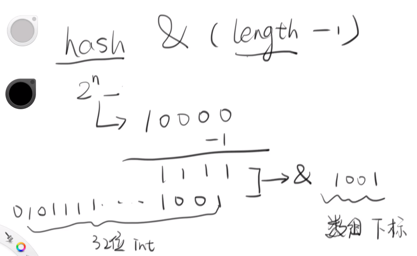
答: 因为它需要计算未来丢进来的元素应该被放到哪个桶里,比如你现在有16个桶
在源码中有这么一个函数,它拿这个元素的哈希值按位与上一个桶的数量(容量)-1
这样就能够计算出它应该被放在哪个桶里(这个元素对应的数组下标),
在哈希表中的对应下标,你可以把它看成一个数组
1
2
3
4
|
static int indexFor(int h, int length) {
    // Hash value of key & (array length - 1)
    return h & (length-1);
}
|
那么为什么默认容量必须是2的n次方呢?从下图我们可以看到,因为只有它的长度是
2的n次方的时候,才能保证对它-1操作拿到的全部是1的值(二进制),这样对它按位
与,才能够非常快速的计算出它的数组下标(桶),并且它的分布还是均匀的
它会给你默认向上取整成2的n次方,如下源码所示
 1
 2
 3
 4
 5
 6
 7
 8
 9
10
11
12
13
14
|
private static int roundUpToPowerOf2(int number) {
    // assert number >= 0 : "number must be non-negative";
    return number >= MAXIMUM_CAPACITY
            ? MAXIMUM_CAPACITY
            : (number > 1) ? Integer.highestOneBit((number - 1) << 1) : 1;
}

private void inflateTable(int toSize) {
    // Find a power of 2 >= toSize
    int capacity = roundUpToPowerOf2(toSize);
    threshold = (int) Math.min(capacity * loadFactor, MAXIMUM_CAPACITY + 1);
    table = new Entry[capacity];
    initHashSeedAsNeeded(capacity);
}
|
1
|
static final float DEFAULT_LOAD_FACTOR = 0.75f;
|
- 当元素个数超过
容量*负载因素时就开始扩容,例如默认容量16 * 0.75 = 12那么它会在超过12个元素时给你扩容
1
2
3
4
5
6
7
8
9
|
void addEntry(int hash, K key, V value, int bucketIndex) {
    // threshold 阈值 = 容量 * 负载因素
    if ((size >= threshold) && (null != table[bucketIndex])) {
        resize(2 * table.length);
        hash = (null != key) ? hash(key) : 0;
        bucketIndex = indexFor(hash, table.length);
    }
    createEntry(hash, key, value, bucketIndex);
}
|
对所有的元素重新计算哈希值,然后把它们都重新移动到新的哈希表中,新的容量是旧的容量的2倍
 1
 2
 3
 4
 5
 6
 7
 8
 9
10
11
12
13
14
15
16
17
|
void resize(int newCapacity) {
    Entry[] oldTable = table;
    int oldCapacity = oldTable.length;
    if (oldCapacity == MAXIMUM_CAPACITY) {
        threshold = Integer.MAX_VALUE;
        return;
    }
    //The above code is to record the old array table and save it
	//Create a new 32 capacity array newTable
    Entry[] newTable = new Entry[newCapacity];
    //Put the elements on the oldTable on the newTable to complete the array transfer
    transfer(newTable, initHashSeedAsNeeded(newCapacity));
    //Assign new array to old array after transfer
    table = newTable;
    //Recalculate threshold 32 * 0.75
    threshold = (int)Math.min(newCapacity * loadFactor, MAXIMUM_CAPACITY + 1);
}
|
 1
 2
 3
 4
 5
 6
 7
 8
 9
10
11
12
13
14
15
16
17
18
19
20
21
22
23
|
void transfer(Entry[] newTable, boolean rehash) {
    int newCapacity = newTable.length;
    // 遍历旧表里的每一个桶
    for (Entry<K,V> e : table) {
        while(null != e) {
            // 用 next 取得要转移那个元素的下一个,
            Entry<K,V> next = e.next;
            if (rehash) {
                e.hash = null == e.key ? 0 : hash(e.key); // 计算新的hash值
            }
            // 然后看看 e 在新表中的什么地方
            int i = indexFor(e.hash, newCapacity);
            // 把 e 的下一个元素设置为新表中对应位置的节点
            // 如果没有发生碰撞,那么这个节点为null,当发生碰撞时,next就会链接到已存在的节点上
            // 这是一个典型的链表结构
            e.next = newTable[i];
            // 将 e 转移到新哈希表的头部,使用头插法插入节点
            newTable[i] = e;
            e = next;
            // 经过这几步会发现转移的时候是逆序的, A->B->C迁移后会变成C->B->A,HashMap 的死锁问题就出在这个transfer()函数上
        }
    }
}
|
Java 8 的 HashMap 中开头就有这样几段注释说明
 1
 2
 3
 4
 5
 6
 7
 8
 9
10
11
12
13
14
15
16
17
18
19
20
21
22
23
24
25
26
27
28
29
30
31
32
33
34
35
36
37
38
39
40
41
42
43
44
45
46
47
|
/*
 * Implementation notes.
 *
 * This map usually acts as a binned (bucketed) hash table, but
 * when bins get too large, they are transformed into bins of
 * TreeNodes, each structured similarly to those in
 * java.util.TreeMap. Most methods try to use normal bins,
 * ......
 * 这个Map通常使用的是基于桶的Hash表,但是,当这个桶变得特别大的时候,
 * 它们会被转化成TreeNodes的桶,其中每一个TreeNode都和TreeMap相似(红黑树)
 * 绝大多数情况下,都会尝试使用正常的桶
*/

/*
 * Because TreeNodes are about twice the size of regular nodes, we
 * use them only when bins contain enough nodes to warrant use
 * (see TREEIFY_THRESHOLD). And when they become too small (due to
 * removal or resizing) they are converted back to plain bins.  In
 * usages with well-distributed user hashCodes, tree bins are
 * rarely used.  Ideally, under random hashCodes, the frequency of
 * nodes in bins follows a Poisson distribution
 * (http://en.wikipedia.org/wiki/Poisson_distribution) with a
 * parameter of about 0.5 on average for the default resizing
 * threshold of 0.75, although with a large variance because of
 * resizing granularity. Ignoring variance, the expected
 * occurrences of list size k are (exp(-0.5) * pow(0.5, k) /
 * factorial(k)). The first values are:
 *
 * 0:    0.60653066
 * 1:    0.30326533
 * 2:    0.07581633
 * 3:    0.01263606
 * 4:    0.00157952
 * 5:    0.00015795
 * 6:    0.00001316
 * 7:    0.00000094
 * 8:    0.00000006
 * more: less than 1 in ten million
 *
 * 因为红黑树的树节点是常规节点的几乎两倍大,所以我们只有在这个桶里有足够多的元素的时候
 * 才会使用它们,请参看 TREEIFY_THRESHOLD(转化成树的阈值),当它们变得特别小的时候
 * 它们会被转化回基于链表的桶,如果用户的 hashCode 分布非常均匀的话,那么基于红黑树的桶
 * 很少被用到,理想情况下,在完全随机的 hashCode 的实现中的时候,这个桶中的节点的分布遵从
 * 泊松分布(http://en.wikipedia.org/wiki/Poisson_distribution),它们服从参数是0.5
 * 的泊松分布
 */
static final int TREEIFY_THRESHOLD = 8;
|
- 因为它们遵从泊松分布, 在一个桶里由8个元素的概率是0.00000006,如果这个概率都达到了,那么就应该转化成红黑树了
但这并不意味着Java 8中的HashMap就是完美的,它一样是线程不安全的,这一点要谨记